Friday, September 7, 2018

Count Number of Words in a Cell

Count Number of Words in a Cell


Generic formula 
=LEN(TRIM(CELL))-LEN(SUBSTITUTE(Cell," ",""))+1
Explanation 
Simple trick behind this formula to get the number of words in a cell is we substract the length string without spaces from the length of string with normal spaces and add 1.
In the example shown, the formula in C3 is:
=LEN(TRIM(A1))-LEN(SUBSTITUTE(A1," ",""))+1
How this formula works
TRIM function returns a string with leading spaces, extra spaces and trailing spaces removed. In the example, I give 2 Leading spaces, 3 extra space and 2 trailing space and get removed by TRIM
=TRIM(A1)

To get the length of the string with normal spaces, we combine the LEN and TRIM function.
=LEN(TRIM(A1))

The SUBSTITUTE function replaces existing text with new text in a text string. 
We use the SUBSTITUTE function to get the string without spaces.
=SUBSTITUTE(A1," ","")
To get the length of the string without spaces, we combine the LEN and SUBSTITUTE function.
=LEN(SUBSTITUTE(A1," ",""))
Now comes the simple trick. 
To get the number of words, we subtract the length of the string without spaces (10) from the length of the string with normal spaces (12) and add 1.
=LEN(TRIM(A1))-LEN(SUBSTITUTE(A1," ","")) + 1

Simple, isn't it! 

Thursday, September 6, 2018

Student t - Test in Excel

t-Test

The example can teach you how to perform a t-Test in Excel. The t-Test is used to test the null hypothesis that the means of two populations are equal.
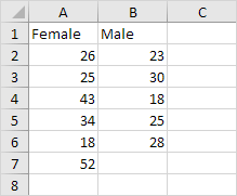
Below you can find the study hours of 6 female students and 5 male students.
H0: μ1 - μ2 = 0
H1: μ1 - μ2 ≠ 0
t-Test in Excel
To perform a t-Test, execute the following steps.
1. First, perform an F-Test to determine if the variances of the two populations are equal. This is not the case, because two populations are not equal here 😊.
2. On the Data tab, in the Analysis group, click Data Analysis.
Click Data Analysis
Note: can't find the Data Analysis button? Click here to load the Analysis ToolPak add-in.
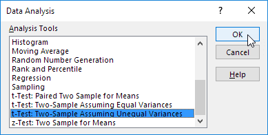
3. Select t-Test: Two-Sample Assuming Unequal Variances and click OK.
Select t-Test: Two-Sample Assuming Unequal Variances
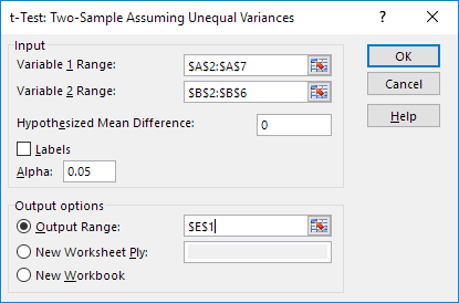
4. Click in the Variable 1 Range box and select the range A2:A7.
5. Click in the Variable 2 Range box and select the range B2:B6.
6. Click in the Hypothesized Mean Difference box and type 0 (H0: μ1 - μ2 = 0).
7. Click in the Output Range box and select cell E1.
t-Test Parameters
8. Click OK.
Result:
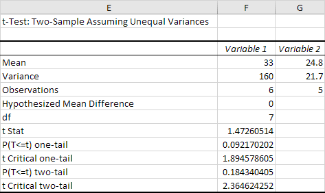
t-Test Result in Excel
Conclusion: We do a two-tail test (inequality). lf t Stat < -t Critical two-tail or t Stat > t Critical two-tail, we reject the null hypothesis. This is not the case, -2.365 < 1.473 < 2.365. Therefore, we do not reject the null hypothesis. The observed difference between the sample means (33 - 24.8) is not convincing enough to say that the average number of study hours between female and male students differ significantly.

Analysis ToolPak in Excel

Analysis ToolPak

The Analysis ToolPak is an Excel add-in program that provides data analysis tools for financial, statistical and engineering data analysis.
To load the Analysis ToolPak add-in, execute the following steps.
1. On the File tab, click Options.

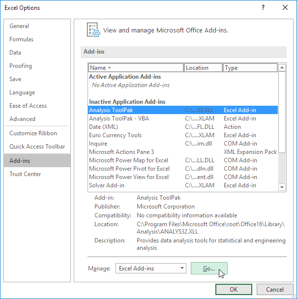
2. Under Add-ins, select Analysis ToolPak and click on the Go button.
Click Analysis ToolPak
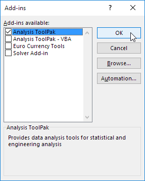
3. Check Analysis ToolPak and click on OK.
Check Analysis ToolPak
4. On the Data tab, in the Analysis group, you can now click on Data Analysis.
Click Data Analysis

Great! You are now ready to do Data analysis in Excel. Click here for Simplest t Test analysis in Excel

Tuesday, September 4, 2018

Check if Cell contains alpha or numeric characters

Check if Cell contains alpha or numeric characters


Generic formula 
=SUMPRODUCT(SEARCH(MID(Cell,ROW(INDIRECT("1:"&LEN(Cell))),1),"abcdefghijklmnopqrstuvwxyz"))
Explanation 
To check the cell contains only alphabet or numeric characters, we can build up the formula as above.
In the example shown, the formula in C3 is:
=SUMPRODUCT(SEARCH(MID(B3,ROW(INDIRECT("1:"&LEN(B3))),1),"abcdefghijklmnopqrstuvwxyz"))
Note that this formula is doing and "absolute match" against the value "abcdefghijklmnopqrstuvwxyz". So you want to include space character include it in the value.

How this formula works

The core of this formula is SUMPRODUCT, which is simply retrieving a value from the array and provide the sum of the values.
=SUMPRODUCT(array)
To get the array value, we use SEARCH, configured for match the characters in the cell, against the given alphabet value, and return the array of number of the position of the alphabet in the value.
=SEARCH(MID(B3,ROW(INDIRECT("1:"&LEN(B3))),1),"abcdefghijklmnopqrstuvwxyz") // search the character against the value
LEN function get the number of character in the cell. 
=LEN(B3)
INDIRCT function returns number of times ROW function to be checked.
=ROW(INDIRECT("1:"&2)
MID function will now turn into array function and check each character of the word in 
the cell against the value and return the number of the position of the character.

=MID(B3,{$1:$2},1)
This formula returns #VALUE! error if B3 contains any non-letter characters and Number if B3 contains only letters or #REF! error if B3 is blank.

You can enclose this formula in an ISNUMBER or ISERR to convert this to a TRUE/FALSE value.

Replace the SEARCH with a FIND to make it case sensitive.

You can put any character in the "abc...xyz" string. This makes it easy to test of alphanumeric, or common punctuation, space etc.

The "1:"&LEN(A1) means that starting from the first letter, all the way to the last letter will be checked. 

Changing that to "2:"&(LEN(A1)-1) will not check the first and last letters.