Excel DATEDIF Function

Summary 

The Excel DATEDIF function returns the difference between two date values in years, months, or days. The DATEDIF (Date + Dif) function is a "compatibility" function that comes from Lotus 1-2-3. For reasons unknown, it is only documented in Excel 2000, but you can use it in your formulas in all Excel versions since that time.

Note: Excel won't help you fill out the arguments for DATEDIF like other functions, but it will work when configured correctly.

Purpose 

Get days, months, or years between two dates

Return value 

A number representing time between two dates

Syntax 

=DATEDIF (start_date, end_date, unit)

Arguments 

• start_date - Start date in Excel date serial number format.
• end_date - End date in Excel date serial number format.
• unit - The time unit to use (years, months, or days).

Usage notes 

The DATEDIF (Date + Dif) function is a "compatibility" function that comes from Lotus 1-2-3. For reasons unknown, it is only documented in Excel 2000, but it works in all Excel versions since that time. As Chip Pearson says: DATEDIF is treated as the drunk cousin of the Formula family. Excel knows it lives a happy and useful life, but will not speak of it in polite conversation.

The DATEDIF function calculates the time between a start_date and an end_date in years, months, or days. The time unit to return is specified using the unit argument, which is supplied as text (upper or lower case).

Examples

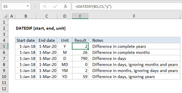
In the example shown, column B contains the date January 1, 2016 and column C contains the date March 1, 2018. In column E:

E5=DATEDIF(B5,C5,"y") // returns 2
E6=DATEDIF(B6,C6,"m") // returns 26
E7=DATEDIF(B7,C7,"d")// returns 790

The table below summarizes available unit values and the result for each:

Unit	Result
"Y"	Difference in complete years
"M"	Difference in complete months
"D"	Difference in days
"MD"	Difference in days, ignoring months and years
"YM"	Difference in months, ignoring days and years
"YD"	Difference in days, ignoring years

Notes

1. Excel will not help you fill in the DATEDIF function like other functions.
2. DATEDIF with throw a #NUM error if start date is greater than the end date. If you are working with a more complex formula where start dates and end dates may be unknown, or out of bounds, you can trap the error with the IFERROR function, or use MIN and MAX to sort out dates.
3. Microsoft recommends not using the "MD" value for unit because it "may result in a negative number, a zero, or an inaccurate result". If you need to calculate days between dates ignoring year and month values, you can use the formula explained here.

Count Number of Words in a Cell

Generic formula 

=LEN(TRIM(CELL))-LEN(SUBSTITUTE(Cell," ",""))+1

Explanation 

Simple trick behind this formula to get the number of words in a cell is we substract the length string without spaces from the length of string with normal spaces and add 1.

In the example shown, the formula in C3 is:

=LEN(TRIM(A1))-LEN(SUBSTITUTE(A1," ",""))+1

How this formula works

TRIM function returns a string with leading spaces, extra spaces and trailing spaces removed. In the example, I give 2 Leading spaces, 3 extra space and 2 trailing space and get removed by TRIM

=TRIM(A1)

To get the length of the string with normal spaces, we combine the LEN and TRIM function.

=LEN(TRIM(A1))

The SUBSTITUTE function replaces existing text with new text in a text string. 



We use the SUBSTITUTE function to get the string without spaces.

=SUBSTITUTE(A1," ","")

To get the length of the string without spaces, we combine the LEN and SUBSTITUTE function.

=LEN(SUBSTITUTE(A1," ",""))







Now comes the simple trick. 



To get the number of words, we subtract the length of the string without spaces (10) from the length of the string with normal spaces (12) and add 1.

=LEN(TRIM(A1))-LEN(SUBSTITUTE(A1," ","")) + 1

Simple, isn't it! 

Student t - Test in Excel

t-Test

The example can teach you how to perform a t-Test in Excel. The t-Test is used to test the null hypothesis that the means of two populations are equal.

Below you can find the study hours of 6 female students and 5 male students.

H₀: μ₁ - μ₂ = 0
H₁: μ₁ - μ₂ ≠ 0

To perform a t-Test, execute the following steps.

1. First, perform an F-Test to determine if the variances of the two populations are equal. This is not the case, because two populations are not equal here 😊.

2. On the Data tab, in the Analysis group, click Data Analysis.

Note: can't find the Data Analysis button? Click here to load the Analysis ToolPak add-in.

3. Select t-Test: Two-Sample Assuming Unequal Variances and click OK.

4. Click in the Variable 1 Range box and select the range A2:A7.

5. Click in the Variable 2 Range box and select the range B2:B6.

6. Click in the Hypothesized Mean Difference box and type 0 (H₀: μ₁ - μ₂ = 0).

7. Click in the Output Range box and select cell E1.

8. Click OK.

Result:

Conclusion: We do a two-tail test (inequality). lf t Stat < -t Critical two-tail or t Stat > t Critical two-tail, we reject the null hypothesis. This is not the case, -2.365 < 1.473 < 2.365. Therefore, we do not reject the null hypothesis. The observed difference between the sample means (33 - 24.8) is not convincing enough to say that the average number of study hours between female and male students differ significantly.

Analysis ToolPak in Excel

Analysis ToolPak

The Analysis ToolPak is an Excel add-in program that provides data analysis tools for financial, statistical and engineering data analysis.

To load the Analysis ToolPak add-in, execute the following steps.

1. On the File tab, click Options.

2. Under Add-ins, select Analysis ToolPak and click on the Go button.

3. Check Analysis ToolPak and click on OK.

4. On the Data tab, in the Analysis group, you can now click on Data Analysis.

Great! You are now ready to do Data analysis in Excel. Click here for Simplest t Test analysis in Excel

Check if Cell contains alpha or numeric characters

Generic formula 

=SUMPRODUCT(SEARCH(MID(Cell,ROW(INDIRECT("1:"&LEN(Cell))),1),"abcdefghijklmnopqrstuvwxyz"))

Explanation 

To check the cell contains only alphabet or numeric characters, we can build up the formula as above.

In the example shown, the formula in C3 is:

=SUMPRODUCT(SEARCH(MID(B3,ROW(INDIRECT("1:"&LEN(B3))),1),"abcdefghijklmnopqrstuvwxyz"))

Note that this formula is doing and "absolute match" against the value "abcdefghijklmnopqrstuvwxyz". So you want to include space character include it in the value.

How this formula works

The core of this formula is SUMPRODUCT, which is simply retrieving a value from the array and provide the sum of the values.

=SUMPRODUCT(array)

To get the array value, we use SEARCH, configured for match the characters in the cell, against the given alphabet value, and return the array of number of the position of the alphabet in the value.

=SEARCH(MID(B3,ROW(INDIRECT("1:"&LEN(B3))),1),"abcdefghijklmnopqrstuvwxyz") // search the character against the value

LEN function get the number of character in the cell. 

=LEN(B3)

INDIRCT function returns number of times ROW function to be checked.

=ROW(INDIRECT("1:"&2)

MID function will now turn into array function and check each character of the word in 

the cell against the value and return the number of the position of the character.

=MID(B3,{$1:$2},1)

This formula returns #VALUE! error if B3 contains any non-letter characters and Number if B3 contains only letters or #REF! error if B3 is blank.

You can enclose this formula in an ISNUMBER or ISERR to convert this to a TRUE/FALSE value.

Replace the SEARCH with a FIND to make it case sensitive.

You can put any character in the "abc...xyz" string. This makes it easy to test of alphanumeric, or common punctuation, space etc.

The "1:"&LEN(A1) means that starting from the first letter, all the way to the last letter will be checked. 

Changing that to "2:"&(LEN(A1)-1) will not check the first and last letters.

How to identify missing numbers sequence in Excel

Identify Missing Numbers Sequence With IF Formula

As we all known, most of sequence numbers are with fixed increment of 1, such as 1, 2, 3, …, N. Therefore, if you can identify the number is not less 1 than its following number, there is a missing number.

We will show you the tutorials with an example as following screenshot shows:

1. In a blank cell, enter the formula of =IF(A3-A2=1,"","Missing"), and press the Enter key. In this case, we enter the formula in Cell B2.

If there is no missing numbers, this formula will return nothing; if missing numbers exist, it will return the text of "Missing" in active cell.

2. Select the cell B2 and drag the fill handle over the range of cells that you want to contain this formula. Now it identifies the missing numbers with the text of "Missing" in corresponding cells of Column B. See the following screenshot:

---

Identify Missing Numbers Sequence With An Array Formula

Sometimes it requires not only identifying missing numbers sequence, but also listing missing numbers too. You can deal it with following steps:

1. in the adjacent cell, please enter the formula = SMALL(IF(ISNA(MATCH(ROW(A$1:A$30),A$1:A$30,0)),ROW(A$1:A$30)),ROW(A1))

A1:A30 = range of numbers, the sequence to check against is from 1 to 30

2. Press the Ctrl + Shift + Enter Keys together to finish the formula. Copy down the formula until you get #NUM! errors meaning all missing numbers have been listed. See screenshot:

---

Re Enable Insert row / Column option

All the sudden, MS Excel's insert Row / Column option is disabled after right clicking. 

I have tried using Excel options, but it's not working. How do I enable it?

Answer is simple. Just follow the steps.

1. Close all open Excel windows

2. In Windows Explorer, go to directory "%appdata%\Microsoft\Excel"

3. Rename the file:  Excel15.xlb --> Excel15.old

Voila! Now, Open the Excel and try to insert the row / column. It will be re enabled now.