How to identify missing numbers sequence in Excel

Identify Missing Numbers Sequence With IF Formula

As we all known, most of sequence numbers are with fixed increment of 1, such as 1, 2, 3, …, N. Therefore, if you can identify the number is not less 1 than its following number, there is a missing number.

We will show you the tutorials with an example as following screenshot shows:

1. In a blank cell, enter the formula of =IF(A3-A2=1,"","Missing"), and press the Enter key. In this case, we enter the formula in Cell B2.

If there is no missing numbers, this formula will return nothing; if missing numbers exist, it will return the text of "Missing" in active cell.

2. Select the cell B2 and drag the fill handle over the range of cells that you want to contain this formula. Now it identifies the missing numbers with the text of "Missing" in corresponding cells of Column B. See the following screenshot:

---

Identify Missing Numbers Sequence With An Array Formula

Sometimes it requires not only identifying missing numbers sequence, but also listing missing numbers too. You can deal it with following steps:

1. in the adjacent cell, please enter the formula = SMALL(IF(ISNA(MATCH(ROW(A$1:A$30),A$1:A$30,0)),ROW(A$1:A$30)),ROW(A1))

A1:A30 = range of numbers, the sequence to check against is from 1 to 30

2. Press the Ctrl + Shift + Enter Keys together to finish the formula. Copy down the formula until you get #NUM! errors meaning all missing numbers have been listed. See screenshot:

---

Re Enable Insert row / Column option

All the sudden, MS Excel's insert Row / Column option is disabled after right clicking. 

I have tried using Excel options, but it's not working. How do I enable it?

Answer is simple. Just follow the steps.

1. Close all open Excel windows

2. In Windows Explorer, go to directory "%appdata%\Microsoft\Excel"

3. Rename the file:  Excel15.xlb --> Excel15.old

Voila! Now, Open the Excel and try to insert the row / column. It will be re enabled now.

Quickly replace multiple space characters with a tab character

Replacing multiple spaces with a tab can be a nightmare, unless you know this simple Find and Replace trick.

Word processing has been around for a long time, and the techniques seem ingrained in our psyche. Yet every once in a while, I run across a document that uses multiple spaces instead of tabs to align text. The result is often a big mess. There are three ways to fix this problem:

• Manually replace the multiple space characters with tabs.
• Use several Find and Replace tasks, which is a bit faster than doing it manually.
• Use one Find and Replace task to replace each instance of multiple space characters with a single tab character.

I know which one I’d choose! To replace multiple and consecutive spaces with a single tab character, do the following:

1. Choose Replace from the Edit menu (or press [Ctrl]+H) to open the Find And Replace dialog box.
2. Click the More button.
3. In the Find What text box, enter one space character and the following characters, exactly as shown: {2,}.
4. In the Replace With control, enter ^t.
5. Check the Use Wildcards option. 
   
6. Click Replace All.
7. Click Close.

The {2,} component tells Word to find two or more of the literal character, which in this case is a space character. You could use this component to find other multiple characters. The ^t component represents a single tab. To replace the spaces with more than one tab, simply add one ^t component for each additional tab. Keep in mind that this technique will replace every occurrence of multiple and consecutive space characters, including some you might not want to replace with a tab. If you want to retain a legitimate occurrence of multiple spaces, select only the text that you want to run the Find and Replace task against before executing it. Or click Find Next so you can review the occurrence to decide whether you want to replace it or not. This replace trick will work in any Office application, not just Word.

Two-way lookup with INDEX and MATCH

Generic formula 

=INDEX(data,MATCH(val,rows,1),MATCH(val,columns,1))

Explanation 

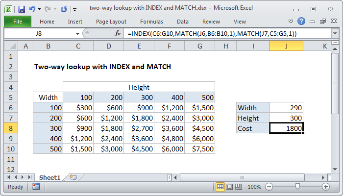
To lookup in value in a table using both rows and columns, you can build a formula that does a two-way lookup with INDEX and MATCH.

In the example shown, the formula in J8 is:

=INDEX(C6:G10,MATCH(J6,B6:B10,1),MATCH(J7,C5:G5,1))

Note that this formula is doing and "approximate match", so row values and column values must be sorted.

How this formula works

The core of this formula is INDEX, which is simply retrieving a value from C6:G10 (the "data") based on a row number and a column number.

=INDEX(C6:G10, row, column)

To get the row and column numbers, we use MATCH, configured for approximate match, by setting the 3rd argument to 1 (TRUE):

MATCH(J6,B6:B10,1) // get row number
MATCH(J7,C5:G5,1) // get column number

In the example, MATCH will return 2 when width is 290, and 3 when height is 300.

In the end, the formula reduces to:

=INDEX(C6:G10, 2, 3)
= 1800

Two-way lookup with VLOOKUP

Generic formula 

=VLOOKUP(lookup_value,table,MATCH(col_name,col_headers,0),0)

Explanation 

Preface

Inside the VLOOKUP function, the column index argument is normally hard-coded as a static number.  However, you can also create a dynamic column index by using the MATCH function to locate the right column. This technique allows you to create a dynamic two-way lookup, matching on both rows and columns. It can also make a VLOOKUP formula more resilient: VLOOKUP can break when columns are inserted or removed from a table, but a formula with VLOOKUP + MATCH can continue to work correctly even changes are made to columns.

Example

In the example, we are using this formula to dynamically lookup both rows and columns with VLOOKUP:

=VLOOKUP(H2,B3:E11,MATCH(H3,B2:E2,0),0)

H2 supplies the lookup value for the row, and H3 supplies the lookup value for the column.

How this formula works

This is a standard VLOOKUP exact match formula with one exception: the column index is supplied by the MATCH function.

Note that the lookup array given to MATCH (B2:E2) representing column headers deliberately includes the empty cell B2. This is done so that the number returned by MATCH is in sync with the table used by VLOOKUP. In other words, you need to give MATCH a range that spans the same number of columns VLOOKUP is using in the table. In the example (for Feb) MATCH returns 3, so after MATCH runs, the VLOOKUP formula looks like this:

=VLOOKUP(H2,B3:E11,3,0)

Which returns sales for Colby (row 4) in Feb (column 3), which is $6,786.